    Augmented Dickey-Fuller Test

data:  rw_series
Dickey-Fuller = -1.8871, Lag order = 4, p-value = 0.6234
alternative hypothesis: stationary15 Stationarity and Differencing
15.1 Introduction
In the previous chapter, we introduced the idea of time series data and explored some its key components.
This chapter develops those ideas by reviewing the concepts of stationarity and differencing. These are fundamental concepts in time series analysis that help us understand the nature of our data and prepare it for predictive modelling.
15.1.1 Stationarity
A time series is considered stationary when its statistical properties remain constant over time.
Specifically, its mean, variance, and autocorrelation structure shouldn’t change across different time periods.
Here’s an example of two time series. The one on the left is stationary, and the one on the right is non-stationary:
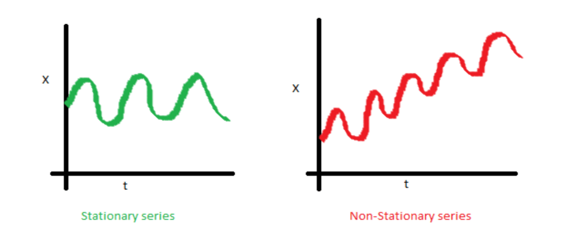
Notice that in the right-hand image, the mean would be different if we sampled the first half of the dataset, compared to the second half. If we did the same thing to the image on the left, we could expect the mean of the first half to be roughly equal to that of the second half.
Understanding stationarity is crucial because most time series models and statistical procedures assume that the data we’re using is stationary. In real-world applications, however, many time series exhibit non-stationary behaviour such as showing trends, seasonal patterns, or varying volatility over time.
15.1.2 Differencing
This is where differencing comes into play. Differencing is a transformation technique we can use to convert non-stationary time series into stationary ones, and therefore make it ready for analysis.
It involves calculating the differences between consecutive observations. First-order differencing can remove linear trends, while second-order differencing can eliminate quadratic trends. Seasonal differencing helps address periodic patterns in the data.
In this chapter, we’ll explore:
How to identify whether a time series is stationary using both visual inspection and statistical tests;
Various transformation techniques to achieve stationarity;
The proper application of differencing and its impact on time series analysis; and
How these concepts extend to more complex multivariate time series.
15.2 What is ‘Stationarity’?
15.2.1 Introduction
In time series analysis (TSA), a stochastic process \(X_t\) is said to be stationary if its statistical properties remain constant over time.
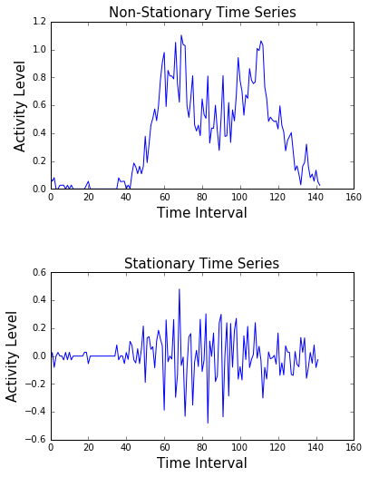
Notice the difference in the two time series plots below. The non-stationary plot has a clear ‘pattern’ to it, while the stationar plot doesn’t.
15.2.2 Types of stationarity
We identify various types of stationarity in time series data, including strict, trend, and difference stationarity.
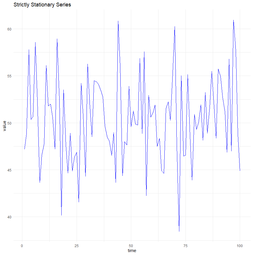
Strict stationarity
Strict stationarity means that the statistical properties of the process generating the time series data do not depend on time at all.
Formally, this is expressed as:
\[ P(Xt1,Xt2,...,Xtn)=P(Xt1+k,Xt2+k,...,Xtn+k) \]
This implies that all moments of the series, such as mean, variance, autocorrelation, etc., are constant over time and don’t depend on the specific time at which the series is observed.
Plotted, a time series with this characteristic would look something like this:
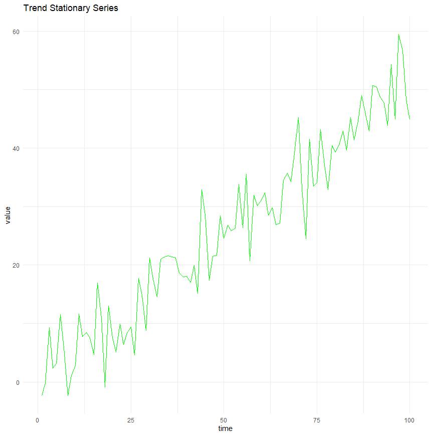
Trend stationarity
Trend stationarity occurs when a time series can have a deterministic trend (linear or otherwise), but the series becomes strictly stationary once this trend is removed.
In other words, the fluctuations around the trend do not depend on time, and their statistical properties remain constant.
This type of series can be made stationary through detrending, i.e., by subtracting the estimated trend from the data.
A time series that fits this criteria would look something like this. Notice that there is a clear trend, but if that trend was to be removed, the series would be stationary:
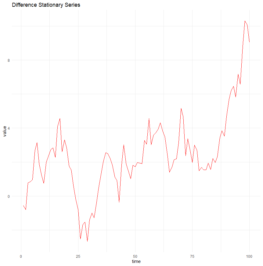
Difference stationarity
Difference stationarity is more complex, and involves time series that become stationary once they are differenced a certain number of times.
Such series often contain one or more unit roots, and differencing helps eliminate these roots, thus stabilising the mean of the series.
A common example is an integrated series of order one, \(I(1)\), which requires one differencing to achieve stationarity.
A time series of this type would look something like this:
15.2.3 Importance of stationarity
Stationarity is really important, because many statistical modelling techniques and forecasting methods in time series analysis rely on the assumption that the underlying properties of the time series data do not change over time.
This is because:
When a series is stationary, its statistical properties like mean and variance remain constant over time, which makes it easier to predict future values based on past data.
Non-stationary data, where mean and variance change, can lead to models that are unreliable and perform poorly in prediction because the conditions under which the model was developed no longer apply.
So, remember that many statistical tests and models assume stationarity because they rely on the assumption that the properties of the series do not change when applying the model or conducting inference. For instance, if the time series has a constant mean, any estimate of the mean will have more validity over time, enabling more accurate and meaningful inferences from historical data to future data.
In terms of predictive modelling, stationarity ensures that the parameters estimated from the time series data are stable and consistent.
- In non-stationary series, the changing underlying patterns can cause parameters of the model (like coefficients in a regression model) to change too, leading to a model that might not work well outside the sample period used for estimation.
Non-stationary data can lead to spurious or misleading statistical relationships, known as “spurious regressions”.
- For example, two independent non-stationary series may appear to be related just because they both trend over time. This can lead to incorrect conclusions about the relationships between variables.
When multiple time series are used together in analysis (e.g., in econometrics), having all series stationary is often necessary.
- Non-stationary series can distort the relationships and interactions among the series, complicating analyses such as cointegration, which are used to identify equilibrium relationships between them.
Because of this, transforming non-stationary data into stationary data is a common practice before further analysis.
We’ll cover this later in the chapter, after considering some approaches to testing for stationarity within our time series data.
15.3 Tests for Stationarity
15.3.1 Introduction
As we’ve discussed, stationarity is a fundamental concept in time series analysis. It refers to a process whose statistical properties, such as mean, variance, and autocorrelation, remain constant over time.
Several formal tests help us assess stationarity, including the Augmented Dickey-Fuller (ADF) test, the Kwiatkowski-Phillips-Schmidt-Shin (KPSS) test, and visual diagnostics such as line plots and rolling statistics.
15.3.2 Augmented Dickey-Fuller (ADF) Test
The Augmented Dickey-Fuller (ADF) test is a widely used hypothesis test for stationarity. It examines whether a time series has a unit root, which indicates non-stationarity.
A ‘unit root’ means the value of the series is highly dependent on its past values. Remember the basic idea that the temperature today is dependent on the temperature yesterday.
The test operates under the following hypotheses:
Null Hypothesis (\(H_0\)): The series has a unit root (i.e., it is non-stationary).
Alternative Hypothesis (\(H_a\)): The series is stationary.
Here is an example of the output of the ADF test in R:
If the p-value is below a chosen significance level (e.g., 0.05), the null hypothesis is rejected, suggesting the series is stationary. Otherwise, we fail to reject the null, indicating non-stationarity.
In this case, with p > 0.05, we would have to conclude that the series is non-stationary, and we’d need to do something about it!
15.3.3 Kwiatkowski-Phillips-Schmidt-Shin (KPSS) Test
The KPSS test is another method for assessing stationarity, but unlike ADF, it has opposite hypotheses:
Null Hypothesis (\(H_0\)): The series is stationary.
*Alternative Hypothesis *(\(H_a\)): The series is non-stationary.
Here is the output from the KPSS test in R:
    KPSS Test for Level Stationarity

data:  rw_series
KPSS Level = 0.95298, Truncation lag parameter = 4, p-value = 0.01
In this case, a significant KPSS test (low p-value) suggests that the series is non-stationary, whereas a non-significant result (high p-value) suggests stationarity.
So the ADF and KPSS tests have confirmed that our time series data is non-stationary.
15.3.4 Visual tests
Formal statistical tests provide p-values and a clear cut-off for what is stationary and non-stationary. However, they can be influenced by sample size and parameter choices.
Visual inspection therefore remains an important tool for detecting stationarity by looking at trends, seasonality, and changing variance.
Key methods include:
- Line plots
- A stationary series should fluctuate around a constant mean with consistent variance. Non-stationary series often show trends, drifts, or changing variance over time.
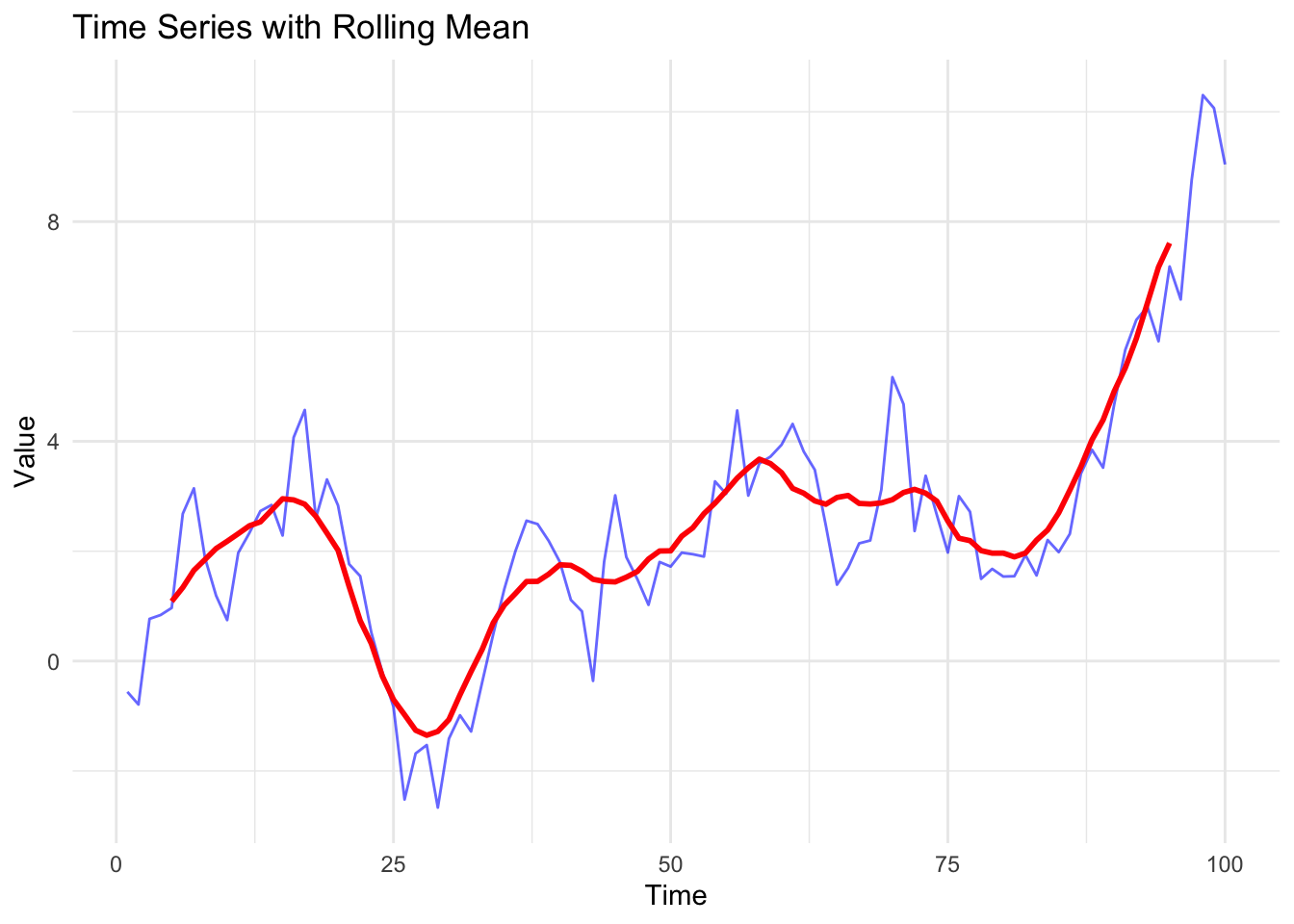
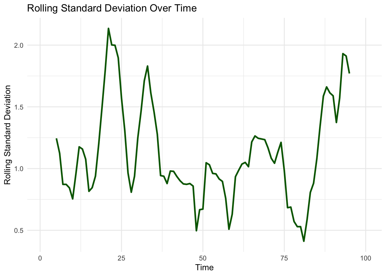
- Rolling Mean and Rolling Standard Deviation
- By computing the moving average and moving standard deviation, we can see whether statistical properties change over time.
In the examples below, we can see that the mean and the standard deviation appear to change over time, which indicates that our data is non-stationary.
15.4 Transformations for Achieving Stationarity
15.4.1 Introduction
We’ve noted that many time series models assume stationarity, meaning that the statistical properties of the series (such as mean and variance) remain constant over time.
We’ve also noted that real-world time series (including those in sport) often exhibit trends, changing variance, or seasonality, making them non-stationary.
To make a series stationary, we need to apply mathematical transformations that remove trends, stabilise variance, and/or eliminate seasonal patterns.
Common transformation techniques include log transformation for variance stabilisation, differencing for trend removal, and seasonal adjustments for periodic patterns.
15.4.2 Log transformation
A log transformation helps stabilise variance when the magnitude of fluctuations increases over time. This is useful when dealing with data like financial data, population growth, or any data that exhibits exponential growth.
- Before transformation, large fluctuations may obscure patterns in the data.
- After transformation, the scale of the variations is compressed, making trends and seasonality more consistent.
Here’s an example of a time series before, and after, log transformation:
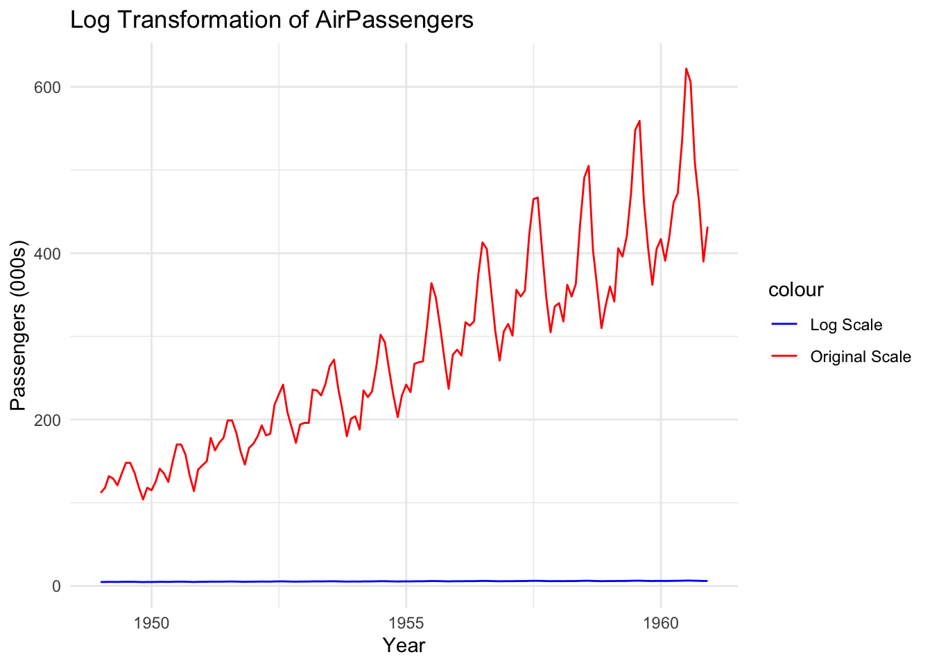
Notice that the red line (original data) shows increasing fluctuations over time. The blue line (log-transformed data) vastly reduces the scale of these fluctuations, making variance more stable.
15.4.3 Differencing for Trend Removal
Differencing removes trends by computing the difference between consecutive observations.
A first-order difference (subtracting each value from the previous one) eliminates linear trends, while a second-order difference removes quadratic trends.
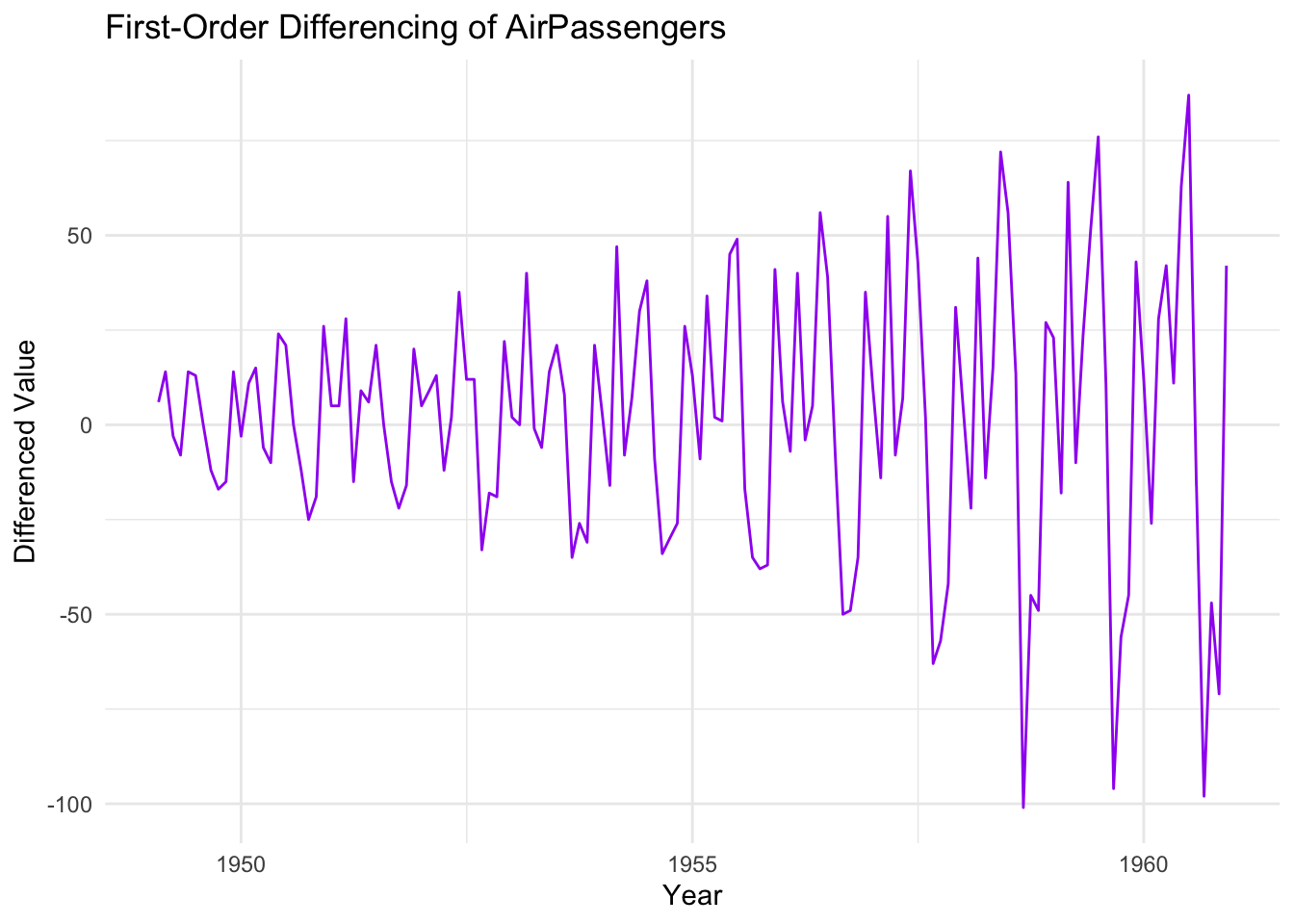
Notice that differencing removes the upward trend we saw in the original data.
However, differencing doesn’t always solve all issues at once. If the differenced series still exhibits patterns, additional differencing or other transformations (e.g., seasonal adjustments) may be needed.
15.4.4 Seasonal Transformation
Time series data often contains seasonal cycles, meaning values at the same time each year or month tend to behave similarly. Removing seasonality makes it easier to analyse underlying trends and random fluctuations.
Methods for Seasonal Adjustment
- Seasonal Differencing: Subtract each observation from its equivalent in the previous cycle (e.g., one year earlier for monthly data).
- Decomposition: Break the series into trend, seasonal, and residual components.
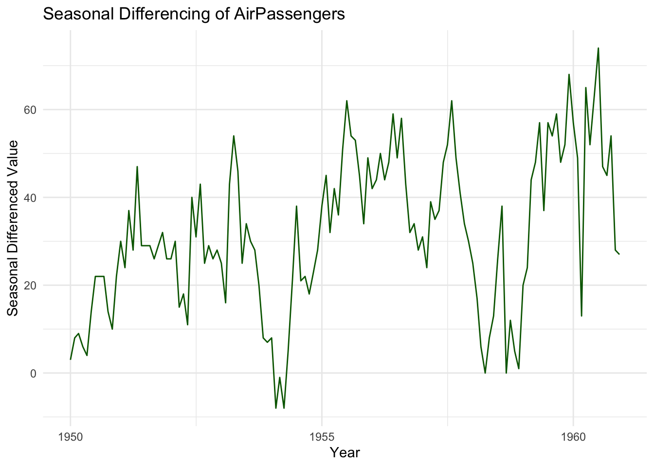
Notice that this transformation removes recurring seasonal effects, making the series more stationary. If patterns persist, further transformations (e.g., log + differencing) may be required.
15.4.5 Conclusion
Transformations help achieve stationarity in time series data by stabilising variance (log transformation), removing trends (differencing), and eliminating seasonal effects (seasonal differencing or decomposition).
15.5 The Role of Differencing
15.5.1 Introduction
Many time series exhibit trends or seasonality, making them non-stationary and unsuitable for traditional forecasting models like ARIMA.
As noted in the previous section, differencing is a key transformation technique used to remove trends and make a time series stationary by computing the difference between consecutive observations.
By stabilising the mean, differencing allows time series models to focus on underlying patterns rather than long-term movements.
However, choosing the right level of differencing is crucial; too little may leave trends in the data, while too much can introduce artificial randomness.
15.5.2 The impact of differencing
Differencing transforms a non-stationary series into a stationary one by subtracting each value from the previous observation. The primary effects of differencing are:
Trend removal: Differencing eliminates linear trends, making it easier to detect seasonal patterns or stochastic fluctuations.
Mean stabilisation: Since a non-stationary series often has a changing mean, differencing creates a series that fluctuates around a constant level.
Enhanced autocorrelation analysis: A differenced series allows for meaningful Autocorrelation Function (ACF) and Partial Autocorrelation Function (PACF) analysis, which are essential for model selection. We introduced ACF in the previous chapter.
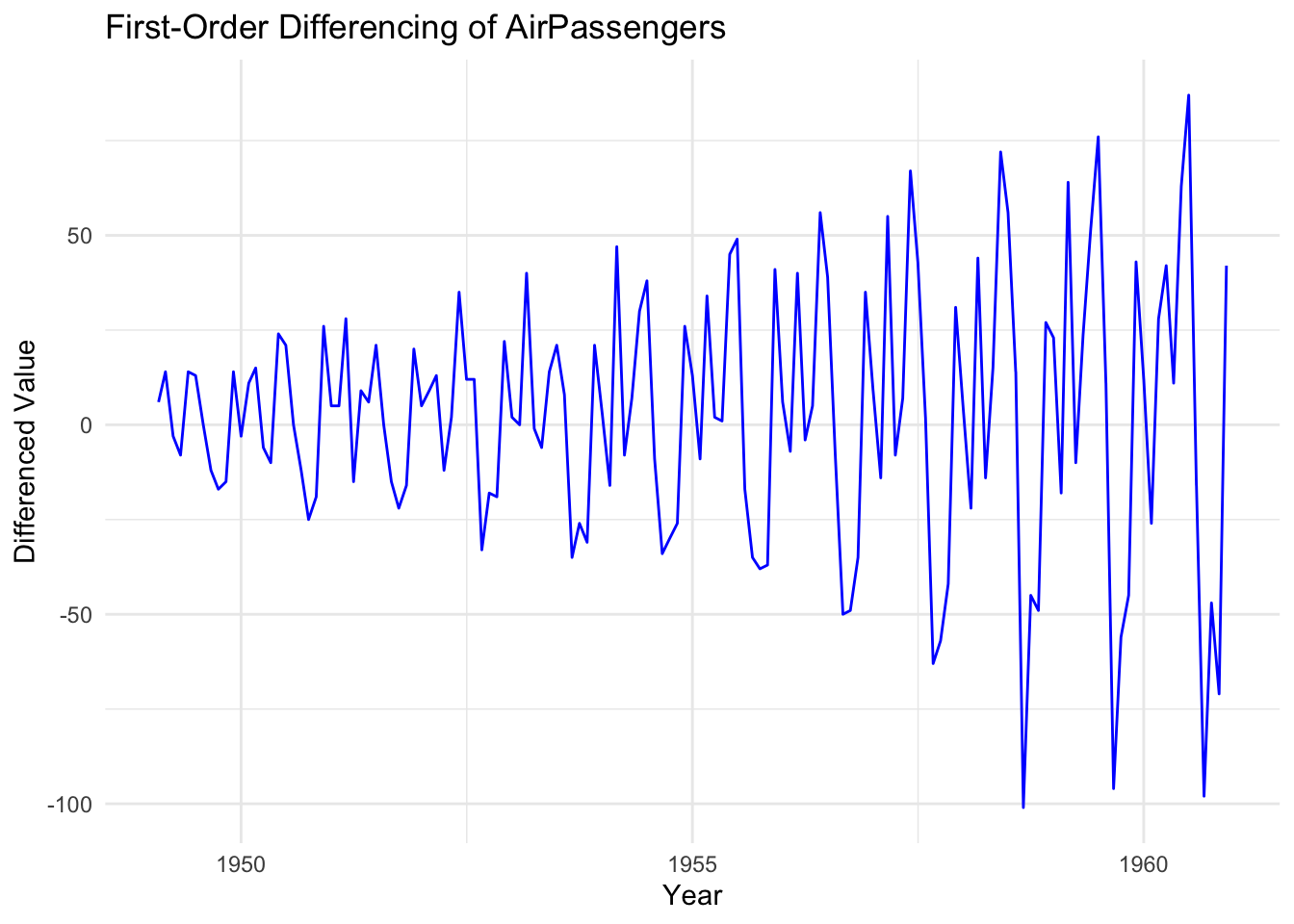
Notice that the original upward trend has been removed. The differenced series fluctuates around a constant mean, indicating that stationarity has been achieved.
15.5.3 The order of differencing
The order of differencing ($d$) refers to the number of times a series is differenced to achieve stationarity. The most common choices are:
First-order differencing (d=1):
Removes linear trend.
Often sufficient for making a series stationary.
Second-order differencing (d=2):
Removes quadratic trends (curved trends).
Used when first-order differencing does not achieve stationarity.
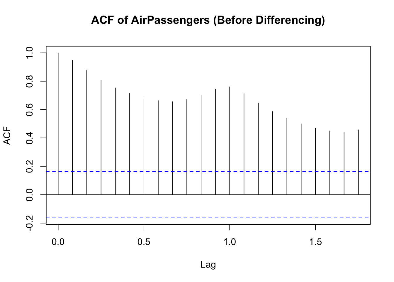
A simple way to determine the necessary differencing order is by examining the ACF plot:
If ACF decreases slowly, the series is likely non-stationary, requiring differencing.
If ACF cuts off quickly, the series may already be stationary.
This first plot shows the ACF before differencing:
The second plot shows what ACF looks like after differencing. Notice the sharp drop-off in the correlation coefficients:

Therefore:
- If the ACF plot of the original series shows slow decay, differencing is needed.
- If the ACF plot of the differenced series quickly drops to zero, first-order differencing was sufficient.
15.6 Stationarity in Multivariate Time Series Data
15.6.1 Introduction
So far, we’ve discussed univariate time series analysis, where we’re interested in one variable or measure.
In multivariate time series analysis, where we are interested in more than one variable over time, stationarity remains crucial for meaningful statistical modeling.
Unlike univariate series, where differencing can remove trends, multivariate time series require additional techniques to ensure stationarity across multiple variables. In particular, when two or more time series are non-stationary but move together over time, cointegration may exist.
This concept allows for meaningful long-term relationships between variables, even if they’re individually non-stationary. Testing for cointegration and applying models such as the Johansen test and Vector Autoregression (VAR) helps to analyse dependencies between multiple time series, and ensure appropriate forecasting.
15.6.2 Cointegration
What Is “Cointegration”?
When two or more non-stationary time series exhibit a stable long-term relationship, they are said to be cointegrated. Even though their individual trends may be stochastic, there exists a linear combination of these variables that is stationary.
For example:
- Stock prices of two companies in the same industry may drift over time but maintain a stable price ratio.
- Exchange rates and interest rates may trend separately but share a long-term equilibrium.
Testing for Cointegration in R
To check for cointegration, we can use the Engle-Granger test or the Johansen test.
The Engle-Granger test works in two steps:
- First, regress one variable on another.
- Then, test the residuals for stationarity.
Notice that the results of the test are reported based on the ADF test we encountered earlier.
    Augmented Dickey-Fuller Test

data:  resid(lm(y2 ~ y1))
Dickey-Fuller = -4.8238, Lag order = 4, p-value = 0.01
alternative hypothesis: stationary
If the ADF test on residuals rejects the null hypothesis (p-value < 0.05), the residuals are stationary, indicating cointegration. This is the case in the output above.
If the test fails to reject the null, the variables do not share a stable relationship.
Remember: we’re checking for cointegration because it allows us to assume that two (or more) variables act ‘as one’ over time, even though they are seperate.
15.6.3 Johansen’s Test
While the Engle-Granger test only tests for one cointegration relationship at a time, the Johansen test (Johansen’s Trace and Maximum Eigenvalue tests) can detect multiple cointegrating relationships in a multivariate system.
How Johansen’s Test Works
- It first determines how many cointegrating relationships exist between time series.
- Then, it tests whether a linear combination of variables is stationary.
Here’s an example of the test in R:
######################
# Johansen-Procedure #
######################

Test type: trace statistic , with linear trend

Eigenvalues (lambda):
[1] 0.4043094 0.0155186

Values of teststatistic and critical values of test:

          test 10pct  5pct  1pct
r <= 1 |  1.53  6.50  8.18 11.65
r = 0  | 52.30 15.66 17.95 23.52

Eigenvectors, normalised to first column:
(These are the cointegration relations)

          y1.l2       y2.l2
y1.l2  1.000000  1.00000000
y2.l2 -1.036377 -0.06746412

Weights W:
(This is the loading matrix)

           y1.l2       y2.l2
y1.d -0.06177683 -0.05586172
y2.d  1.13444082 -0.06325464
The test output shows the number of cointegrating relationships. If the test statistic is greater than the critical value, we reject the null hypothesis and confirm cointegration.
The number of cointegrating relationships (rank) determines how variables interact long-term.
15.6.4 Vector Autoregression (VAR)
Finally Vector Autoregression (VAR) is a statistical model used for multivariate time series forecasting when multiple variables influence each other.
Unlike univariate models (such as ARIMA), VAR models treat all variables as endogenous, meaning each variable depends on past values of both itself and the other variables in the system.
VAR Estimation Results:
=========================
Endogenous variables: y1, y2
Deterministic variables: const
Sample size: 97
Log Likelihood: -339.229
Roots of the characteristic polynomial:
0.6894 0.6894 0.3015 0.3015
Call:
VAR(y = diff_data, p = 2, type = "const")


Estimation results for equation y1:
===================================
y1 = y1.l1 + y2.l1 + y1.l2 + y2.l2 + const

       Estimate Std. Error t value Pr(>|t|)
y1.l1 -0.006602   0.106836  -0.062    0.951
y2.l1 -0.024325   0.037896  -0.642    0.523
y1.l2 -0.096074   0.108899  -0.882    0.380
y2.l2 -0.004048   0.037850  -0.107    0.915
const  0.099478   0.095233   1.045    0.299


Residual standard error: 0.9236 on 92 degrees of freedom
Multiple R-Squared: 0.01665,    Adjusted R-squared: -0.02611
F-statistic: 0.3894 on 4 and 92 DF,  p-value: 0.8158


Estimation results for equation y2:
===================================
y2 = y1.l1 + y2.l1 + y1.l2 + y2.l2 + const

      Estimate Std. Error t value Pr(>|t|)
y1.l1  0.71331    0.26529   2.689  0.00851 **
y2.l1 -0.77151    0.09410  -8.199 1.39e-12 ***
y1.l2 -0.18241    0.27041  -0.675  0.50164
y2.l2 -0.45734    0.09399  -4.866 4.70e-06 ***
const  0.12518    0.23648   0.529  0.59784
---
Signif. codes:  0 '***' 0.001 '**' 0.01 '*' 0.05 '.' 0.1 ' ' 1


Residual standard error: 2.293 on 92 degrees of freedom
Multiple R-Squared: 0.4519, Adjusted R-squared: 0.4281
F-statistic: 18.96 on 4 and 92 DF,  p-value: 2.119e-11


Covariance matrix of residuals:
       y1     y2
y1 0.8530 0.5752
y2 0.5752 5.2598

Correlation matrix of residuals:
       y1     y2
y1 1.0000 0.2715
y2 0.2715 1.0000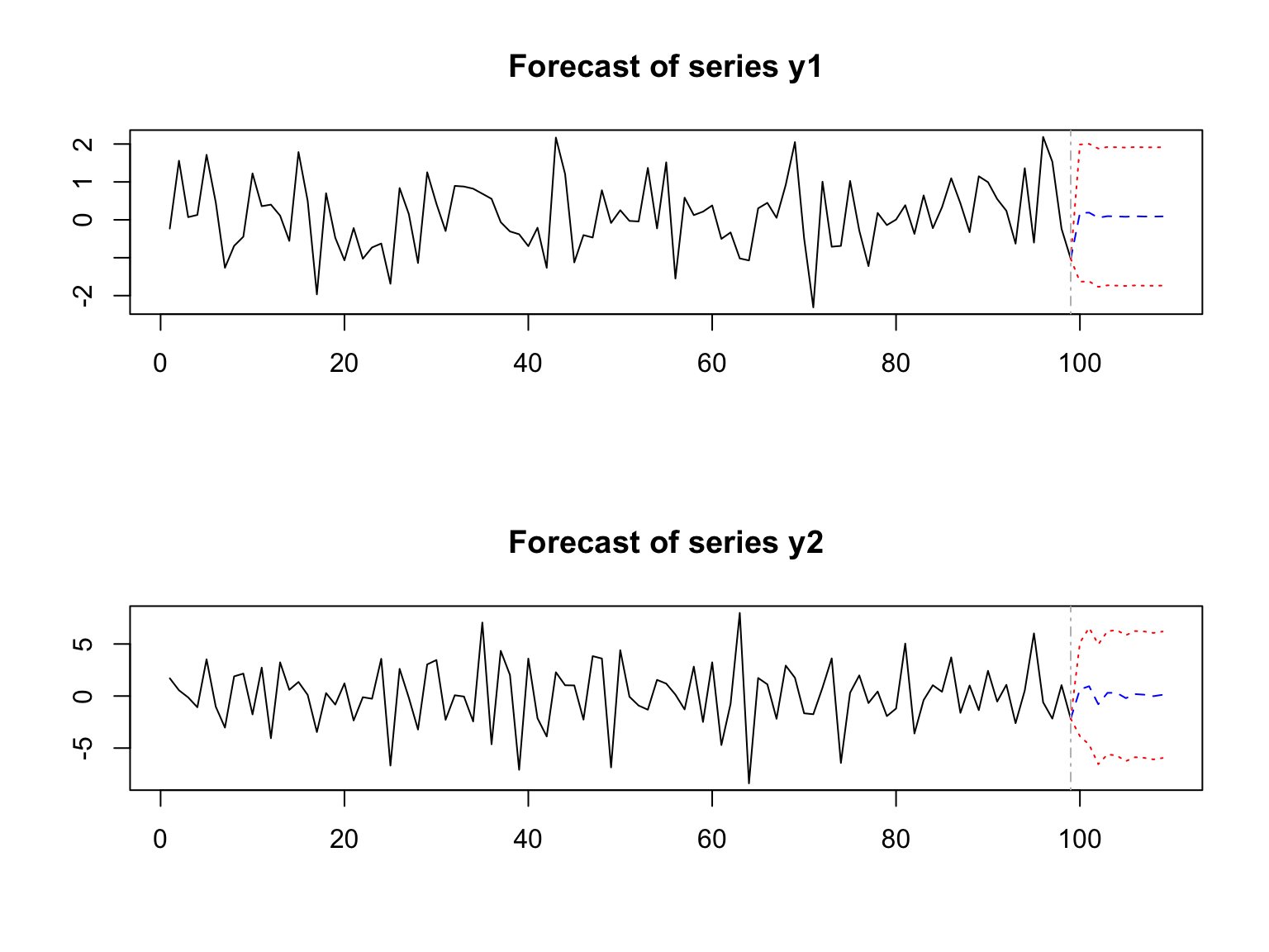
Essentially, the VAR model captures interdependencies between time series variables.
15.7 Conclusion
In this chapter we’ve explored two key concepts in time series analysis, stationarity and differencing. We’ve learned that stationarity can be a problem in time series analysis if we don’t deal with it. Differencing is the way that we address stationarity in our data, making it ready for statistical testing and predictive modelling.